The `meow` Workflow: Visualizing Exposure Control Methods • meow

This vignette shows off the meow framework by walking through running two simulations, one with no item exposure controls and one with item exposure controls. The goal here is examining the workflow, examining the data objects, and showing some possible visualization pathways. We use ggplot2 for the plots and dplyr/tidyr for reshaping; the figures here are pre-rendered so the packages are not required to build the vignette.

# remotes::install_github("klintkanopka/meow")
library(meow)
library(tidyverse)

No exposure controls

First, we’ll set up the simulation with no exposure controls. This requires we select a data loader that defines the simulation data generating process. For a baseline, we’ll just use the built-in data_simple_1pl(). Next, we need to decide how items are selected. Here we use the built-in select_max_info() that picks the next item to maximize Fisher information. Finally, we need an ability update function, and we use update_theta_mle() to treat item parameters are fixed and pre-calibrated and estimate ability after each iteration using maximum likelihood estimation:

out_none <- meow(
  select_fun = select_max_info,
  update_fun = update_theta_mle,
  data_loader = data_simple_1pl,
  init = NULL,
  fix = "item"
)

RMSE of person abilities

After running, we have the out_none object, which is a list with a few different components. First, the $results object is dataframe has one row per iteration, with an estimate and a bias column for every parameter in the simulation, allowing users to track how estimates evolve over the test. Given that we work with simulated data, we can use this to look at the RMSE in ability estimation as a function of the number items administered.

results_none <- out_none$results |>
  mutate(control = "None")

results_none |>
  select(iter, control, starts_with("pers_")) |>
  select(iter, control, ends_with("_bias")) |>
  pivot_longer(ends_with("_bias"), names_to = "person", values_to = "bias") |>
  group_by(iter, control) |>
  summarize(rmse = sqrt(mean(bias^2)), .groups = "drop") |>
  ggplot(aes(x = iter, y = rmse, color = control)) +
  geom_line() +
  labs(x = "Number of Items Delivered", y = "RMSE for Person Ability",
       color = "Exposure Controls") +
  theme_minimal() +
  theme(legend.position = "bottom")

Figure 1

Individual ability bias trajectories may also be of interest:

results_none |>
  select(iter, control, starts_with("pers_")) |>
  select(iter, control, ends_with("_bias")) |>
  pivot_longer(ends_with("_bias"), names_to = "person", values_to = "bias") |>
  ggplot(aes(x = iter, y = bias, color = control, group = person)) +
  geom_line(alpha = 0.4) +
  labs(x = "Number of Items Delivered", y = "Bias in Estimated Person Ability",
       color = "Exposure Controls") +
  theme_minimal() +
  theme(legend.position = "bottom")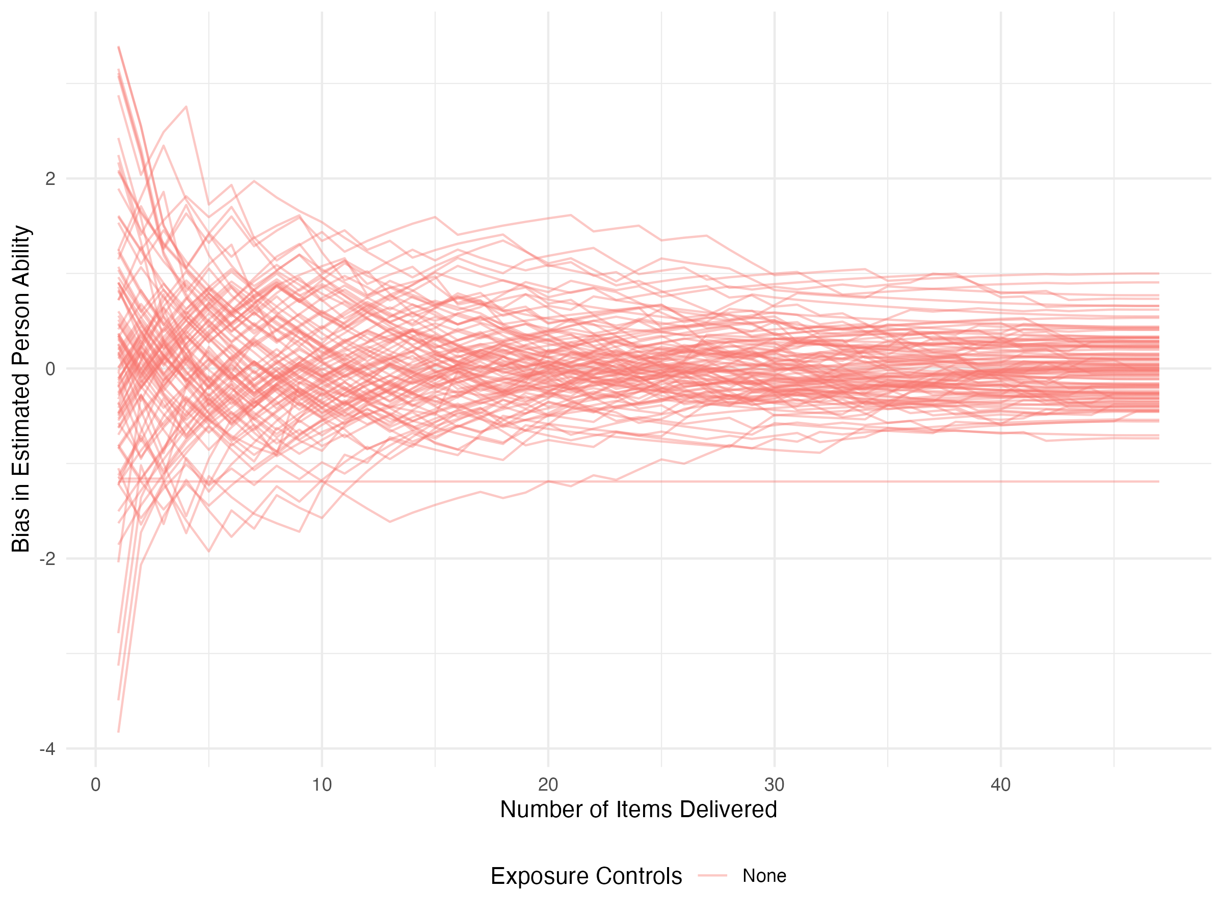

Figure 2

Restricting item exposure

To add a simple exposure control, we write a custom item selection function; this (hopefully easy) expandability is a core feature of meow and a key part of its intended use. To enable this, we’ll use another object exposed to the user: the item-item adjacency matrix. This keeps track of how many times pairs of items have been exposed to the same respondent. Importantly here, the diagonal of the adjacency matrix holds each item’s total exposure count. Our approach will be to convert that to an exposure rate and refuse to administer items whose rate exceeds some user-specified r_max, choosing the most informative item among those that remain.¹

select_restrict_rate <- function(pers, item, R, admin, adj_mat = NULL, r_max = 0.025) {
  # if no items have been administered, give the first five to everyone
  if (!any(admin != 0)) {
    admin[, seq_len(min(5, ncol(admin)))] <- 1L
    return(admin)
  }

  # compute an exposure rate for every item
  exposures <- diag(adj_mat)
  r_obs <- exposures / sum(exposures)
  allowed <- which(r_obs < r_max)

  # 2PL information for every respondent-item combination; column-major
  # recycling avoids materializing extra matrices (matching the package internals)
  n <- nrow(R)
  lin <- (pers$theta - rep(item$b, each = n)) * rep(item$a, each = n)
  p <- stats::plogis(lin)
  info <- matrix(p * (1 - p) * rep(item$a^2, each = n), nrow = n)

  for (i in which(rowSums(admin == 0) > 0)) {
    candidates <- intersect(which(admin[i, ] == 0), allowed)
    if (length(candidates) == 0) next            # no permitted items remain
    admin[i, candidates[which.max(info[i, candidates])]] <- 1L
  }
  admin
}

This selector ships with meow as select_restrict_rate(), so you can use it without defining it yourself; we reproduce it here to show how little code an exposure control takes. We can now conduct a simulation as before, passing a non-default exposure rate through select_args. The modular design ensures the other components of the simulation remain as before, giving comparability between runs.

out_rest <- meow(
  select_fun = select_restrict_rate,
  update_fun = update_theta_mle,
  data_loader = data_simple_1pl,
  init = NULL,
  fix = "item",
  select_args = list(r_max = 0.02)
)

Now let’s compare RMSE across the two conditions:

results_rest <- out_rest$results |>
  mutate(control = "Restricted")

results <- bind_rows(results_none, results_rest)

results |>
  select(iter, control, starts_with("pers_")) |>
  select(iter, control, ends_with("_bias")) |>
  pivot_longer(ends_with("_bias"), names_to = "person", values_to = "bias") |>
  group_by(iter, control) |>
  summarize(rmse = sqrt(mean(bias^2)), .groups = "drop") |>
  ggplot(aes(x = iter, y = rmse, color = control)) +
  geom_line() +
  labs(x = "Number of Items Delivered", y = "RMSE for Person Ability",
       color = "Exposure Controls") +
  theme_minimal() +
  theme(legend.position = "bottom")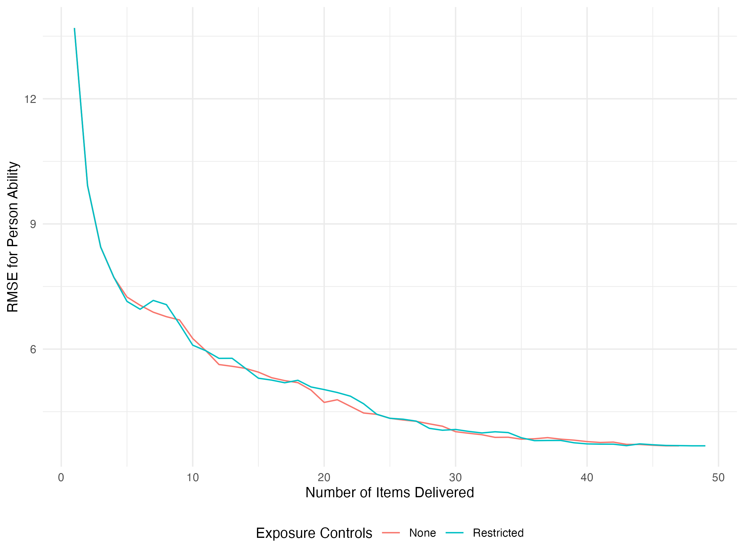

Figure 3

results |>
  select(iter, control, starts_with("pers_")) |>
  select(iter, control, ends_with("_bias")) |>
  pivot_longer(ends_with("_bias"), names_to = "person", values_to = "bias") |>
  filter(iter <= 20) |>
  ggplot(aes(x = iter, y = bias, color = control, group = person)) +
  geom_line(alpha = 0.4) +
  facet_grid(control ~ .) +
  labs(x = "Number of Items Delivered", y = "Bias in Estimated Person Ability",
       color = "Exposure Controls") +
  theme_minimal() +
  theme(legend.position = "bottom")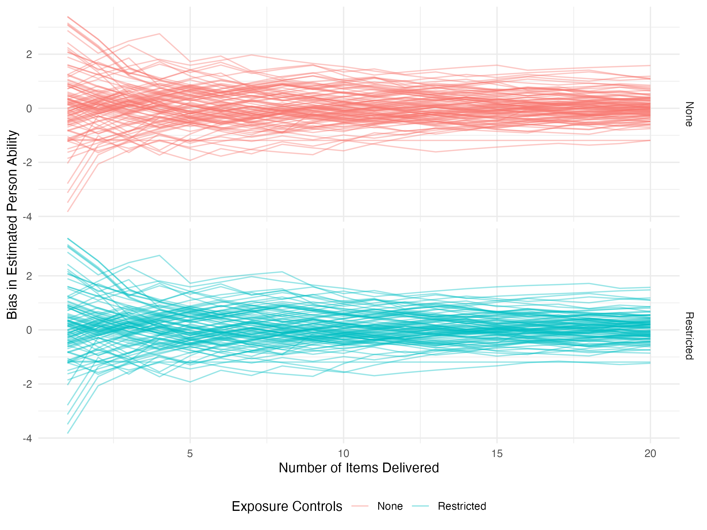

Figure 4

Visualizing the adjacency matrix

One object in meow that’s odd (but powerful) is the adjacency matrix. At the end of a simulation, a list of these is kept in the output object if you want to look at how item exposure evolves over time. The structure of the list of adjacency matrices returned in $adj_mats is designed to make it easy to build dynamic network visualizations of item utilization with statnet and ndtv.

library(statnet)
library(ndtv)

rest_nets <- lapply(out_rest$adj_mats, network)
dyn_rest <- networkDynamic(network.list = rest_nets)

render.d3movie(
  dyn_rest,
  usearrows = FALSE,
  main = "Maximum Fisher Information Item Selection",
  vertex.cex = abs(out_rest$item_tru$b),
  vertex.col = ifelse(out_rest$item_tru$b < 0, "dodgerblue", "tomato")
)