IRT Linking and Gradient Asymmetry: Diagnostic Guide

Background

This document is a diagnostic guide for the frozen expected-count estimator (fit_mixed_subjects). It explains the gradient asymmetry that occurs when the LLM item parameters differ from human parameters and evaluates IRT scale-linking methods as a partial remedy. For the recommended workflow, see the Mixed-Subjects IRT Calibration vignette, which uses fit_mixed_subjects_mml() — the marginal-MML estimator that eliminates the gradient asymmetry without requiring a linking pre-processing step.

Background (frozen expected-count estimator)

A key E-step decision in the frozen expected-count calibration is which item parameters to use when computing posterior quadrature weights for the LLM-generated responses. The frozen estimator uses the same human-calibrated parameters for all three datasets (observed, predicted, generated), which is misspecified when the LLM has different item parameters. This misspecification creates a systematic gradient asymmetry in the combined objective — the correction gradient $\nabla(L_\text{gen} - L_\text{pred})$ is consistently larger than zero because LLM-specific posteriors are more diffuse than human posteriors. The result is a false minimum in the combined loss at unrealistically large discrimination values.

The standard remedy is IRT scale linking: fit a 2PL model to the generated data, transform the LLM parameters onto the human metric, and use those linked parameters for the generated E-step. This document evaluates three classical linking methods:

Method	What is matched
Mean-mean	Mean discrimination and mean difficulty
Mean-sigma	Mean and SD of difficulty
Stocking-Lord	Numerically minimized weighted TCC squared deviation

We characterize both how well each method aligns the LLM parameters to the human scale and — crucially — how the residual misalignment interacts with the power-tuning parameter $\lambda$ .

Linking implementations

The transformation $\theta_\text{human} = A\,\theta_\text{LLM} + B$ implies $a^\dagger = a/A$ and $b^\dagger = Ab + B$ (equivalently $d^\dagger = d - (a/A)B$ ).

library(mixedsubjectsirt)
library(ggplot2)

# Apply (A, B) and return a standardised data frame of item parameters.
# Guards against degenerate linking constants (Inf, NaN, non-positive A) that
# can arise from unusual mirt fits on different platforms.
apply_link <- function(source, A, B, slope_lower = 1e-4) {
  if (!is.finite(A) || A <= 0 || !is.finite(B)) {
    # Degenerate constants: fall back to identity transform
    A <- 1
    B <- 0
  }
  pars <- data.frame(
    item = source$item,
    a    = pmax(slope_lower, source$a / A),
    b    = A * source$b + B,
    stringsAsFactors = FALSE
  )
  # Guard b and d against any residual non-finite values
  pars$b <- ifelse(is.finite(pars$b), pars$b, 0)
  pars$d <- -pars$a * pars$b
  list(pars = pars, A = A, B = B)
}

link_mean_mean <- function(source, target) {
  A <- mean(source$a) / mean(target$a)
  B <- mean(target$b) - A * mean(source$b)
  apply_link(source, A, B)
}

link_mean_sigma <- function(source, target) {
  sd_src <- sd(source$b)
  # If source difficulties have no variance (degenerate mirt fit), fall back
  # to mean-mean linking which does not depend on sd(b).
  if (!is.finite(sd_src) || sd_src < 1e-6) {
    return(link_mean_mean(source, target))
  }
  A <- sd(target$b) / sd_src
  B <- mean(target$b) - A * mean(source$b)
  apply_link(source, A, B)
}

# Stocking-Lord with bounded optimization to prevent item-level overcorrection.
# A is constrained to [0.4, 2.5]; large-variance items can otherwise receive
# inflated linked discriminations that destabilize the downstream M-step.
link_stocking_lord <- function(source, target,
                                theta_grid = seq(-4, 4, by = 0.05),
                                A_bounds   = c(0.4, 2.5),
                                B_bounds   = c(-4,  4)) {
  w <- dnorm(theta_grid) / sum(dnorm(theta_grid))

  tcc <- function(pars, theta) {
    eta <- outer(theta, pars$a, `*`) +
      matrix(pars$d, nrow = length(theta), ncol = nrow(pars), byrow = TRUE)
    rowSums(plogis(eta))
  }

  tcc_target <- tcc(target, theta_grid)

  criterion <- function(params) {
    A <- exp(params[1])
    B <- params[2]
    sum(w * (tcc_target - tcc(apply_link(source, A, B)$pars, theta_grid))^2)
  }

  mm   <- link_mean_mean(source, target)
  init <- c(log(mm$A), mm$B)

  # L-BFGS-B on log(A) keeps A > 0 and enforces the stated bounds
  opt <- optim(
    par     = init,
    fn      = criterion,
    method  = "L-BFGS-B",
    lower   = c(log(A_bounds[1]), B_bounds[1]),
    upper   = c(log(A_bounds[2]), B_bounds[2]),
    control = list(factr = 1e-14, maxit = 1000)
  )

  apply_link(source, exp(opt$par[1]), opt$par[2])
}

rmse <- function(x, y) sqrt(mean((x - y)^2))

Simulation

n_human     <- 400
n_generated <- 1200
n_items     <- 8

true_pars <- data.frame(
  item = paste0("Item", seq_len(n_items)),
  a    = seq(0.8, 1.6, length.out = n_items),
  d    = seq(-1.1, 1.1, length.out = n_items)
)
true_pars$b <- -true_pars$d / true_pars$a

# Human responses
theta_human <- rnorm(n_human)
observed    <- simulate_2pl(theta_human, true_pars)

# LLM: ~10% attenuated discrimination per item, +0.25 logit intercept shift
llm_pars_true <- true_pars
llm_pars_true$a <- pmax(0.4, 0.9 * true_pars$a + rnorm(n_items, 0, 0.05))
llm_pars_true$d <- true_pars$d + 0.25 + rnorm(n_items, 0, 0.15)
llm_pars_true$b <- -llm_pars_true$d / llm_pars_true$a

# Paired predictions and two generated datasets
predicted         <- simulate_2pl(theta_human, llm_pars_true)
generated_matched <- simulate_2pl(rnorm(n_generated),                    llm_pars_true)
generated_shifted <- simulate_2pl(rnorm(n_generated, mean = 0.2, sd = 0.9), llm_pars_true)

The matched sample draws LLM subjects from the same N(0,1) ability distribution as humans. The shifted sample uses mean = 0.2, SD = 0.9, representing a higher-ability, lower-variance LLM response pattern.

Fitting human and LLM models

human_pars       <- fit_2pl(observed,         technical = list(NCYCLES = 500))$pars
llm_raw_matched  <- fit_2pl(generated_matched, technical = list(NCYCLES = 500))$pars
llm_raw_shifted  <- fit_2pl(generated_shifted, technical = list(NCYCLES = 500))$pars

Item parameter summary before linking
Source	mean(a)	sd(a)	mean(b)	sd(b)
True human	1.200	0.280	0.143	0.715
Human MLE	1.357	0.393	0.123	0.708
LLM true (both)	1.077	0.252	-0.093	0.827
LLM raw (matched)	1.079	0.391	-0.046	0.871
LLM raw (shifted)	1.003	0.209	-0.374	0.908

Note the item-level heterogeneity in the LLM parameters. The mean LLM discrimination is ~80% of the human mean, but individual items deviate from this ratio — some LLM items are close to or exceed the human estimate. This heterogeneity means scale-level linking methods cannot perfectly align every item.

Applying the three methods

methods <- c("mean_mean", "mean_sigma", "stocking_lord")

all_links <- list(
  matched = list(
    mean_mean     = link_mean_mean    (llm_raw_matched, human_pars),
    mean_sigma    = link_mean_sigma   (llm_raw_matched, human_pars),
    stocking_lord = link_stocking_lord(llm_raw_matched, human_pars)
  ),
  shifted = list(
    mean_mean     = link_mean_mean    (llm_raw_shifted, human_pars),
    mean_sigma    = link_mean_sigma   (llm_raw_shifted, human_pars),
    stocking_lord = link_stocking_lord(llm_raw_shifted, human_pars)
  )
)

# Linking constants
const_tab <- do.call(rbind, lapply(c("matched", "shifted"), function(case) {
  do.call(rbind, lapply(methods, function(m) {
    data.frame(case = case, method = m,
               A = round(all_links[[case]][[m]]$A, 4),
               B = round(all_links[[case]][[m]]$B, 4))
  }))
}))
knitr::kable(const_tab, row.names = FALSE,
             caption = "Linking constants (A, B)")

Linking constants (A, B)
case	method	A	B
matched	mean_mean	0.7951	0.1592
matched	mean_sigma	0.8123	0.1600
matched	stocking_lord	0.7846	0.1585
shifted	mean_mean	0.7392	0.3993
shifted	mean_sigma	0.7797	0.4144
shifted	stocking_lord	0.7481	0.3741

Parameter alignment after linking

param_tab <- do.call(rbind, lapply(c("matched", "shifted"), function(case) {
  do.call(rbind, lapply(methods, function(m) {
    lp <- all_links[[case]][[m]]$pars
    data.frame(
      case   = case, method = m,
      rmse_a = round(rmse(lp$a, human_pars$a), 4),
      rmse_b = round(rmse(lp$b, human_pars$b), 4),
      max_da = round(max(abs(lp$a - human_pars$a)), 4),
      max_db = round(max(abs(lp$b - human_pars$b)), 4)
    )
  }))
}))
knitr::kable(param_tab, row.names = FALSE,
  col.names = c("Case", "Method", "RMSE(a)", "RMSE(b)", "max|Δa|", "max|Δb|"),
  caption = "Discrepancy between linked LLM parameters and human MLE")

Discrepancy between linked LLM parameters and human MLE
Case	Method	RMSE(a)	RMSE(b)	max\|Δa\|	max\|Δb\|
matched	mean_mean	0.3395	0.2262	0.7025	0.3936
matched	mean_sigma	0.3349	0.2282	0.7248	0.4134
matched	stocking_lord	0.3438	0.2254	0.6884	0.3812
shifted	mean_mean	0.2150	0.1481	0.3379	0.2246
shifted	mean_sigma	0.2288	0.1480	0.4116	0.2655
shifted	stocking_lord	0.2161	0.1501	0.3547	0.2392

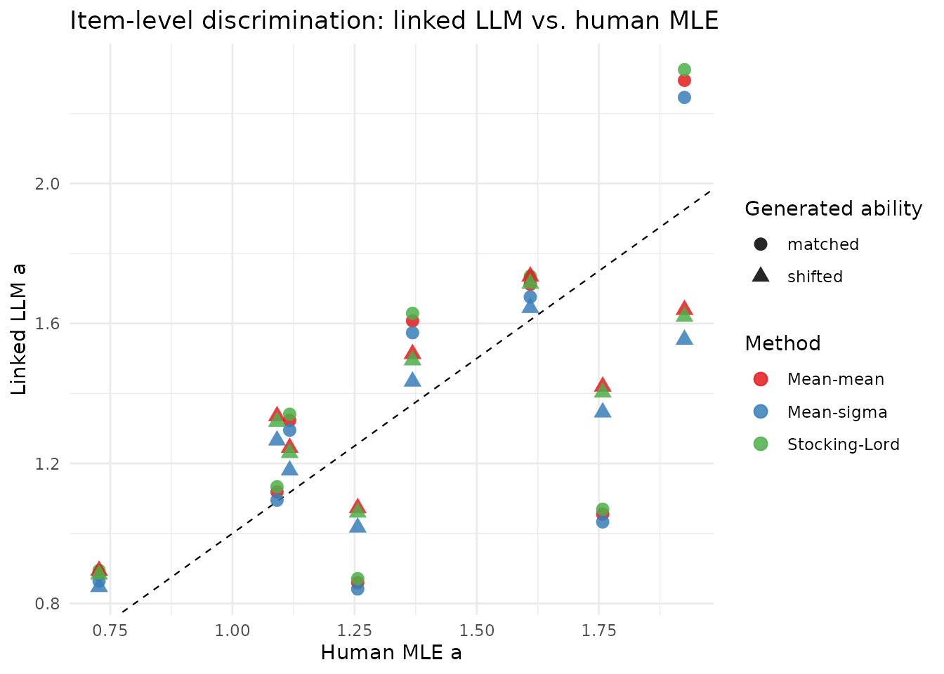
Items deviating most from the 1:1 line are those where the LLM’s discrimination differs most from the human value relative to the group mean — linking cannot individually recalibrate each item.

TCC alignment

theta_seq <- seq(-4, 4, by = 0.1)
tcc_fn <- function(pars, theta) {
  eta <- outer(theta, pars$a, `*`) +
    matrix(pars$d, nrow = length(theta), ncol = nrow(pars), byrow = TRUE)
  rowSums(plogis(eta))
}

# Only show matched case for brevity
tcc_df <- rbind(
  data.frame(theta = theta_seq, tcc = tcc_fn(human_pars, theta_seq),
             method = "Human MLE"),
  data.frame(theta = theta_seq, tcc = tcc_fn(llm_raw_matched, theta_seq),
             method = "LLM unlinked"),
  do.call(rbind, lapply(methods, function(m) {
    data.frame(theta  = theta_seq,
               tcc    = tcc_fn(all_links$matched[[m]]$pars, theta_seq),
               method = m)
  }))
)
tcc_df$method_f <- factor(tcc_df$method,
  levels = c("Human MLE","LLM unlinked","mean_mean","mean_sigma","stocking_lord"),
  labels = c("Human MLE","LLM unlinked","Mean-mean","Mean-sigma","Stocking-Lord"))

ggplot(tcc_df, aes(theta, tcc, colour = method_f, linewidth = method_f,
                   linetype = method_f)) +
  geom_line() +
  scale_colour_manual(values = c(
    "Human MLE"="black","LLM unlinked"="grey60",
    "Mean-mean"="#E41A1C","Mean-sigma"="#377EB8","Stocking-Lord"="#4DAF4A")) +
  scale_linewidth_manual(
    values = c("Human MLE"=1.0,"LLM unlinked"=0.6,
               "Mean-mean"=0.8,"Mean-sigma"=0.8,"Stocking-Lord"=0.8)) +
  scale_linetype_manual(
    values = c("Human MLE"="solid","LLM unlinked"="dashed",
               "Mean-mean"="solid","Mean-sigma"="solid","Stocking-Lord"="solid")) +
  labs(x = "Ability (θ)", y = "Expected score",
       title = "Test characteristic curves — matched ability distribution",
       colour = NULL, linewidth = NULL, linetype = NULL) +
  theme_minimal(base_size = 11) + theme(legend.position = "bottom")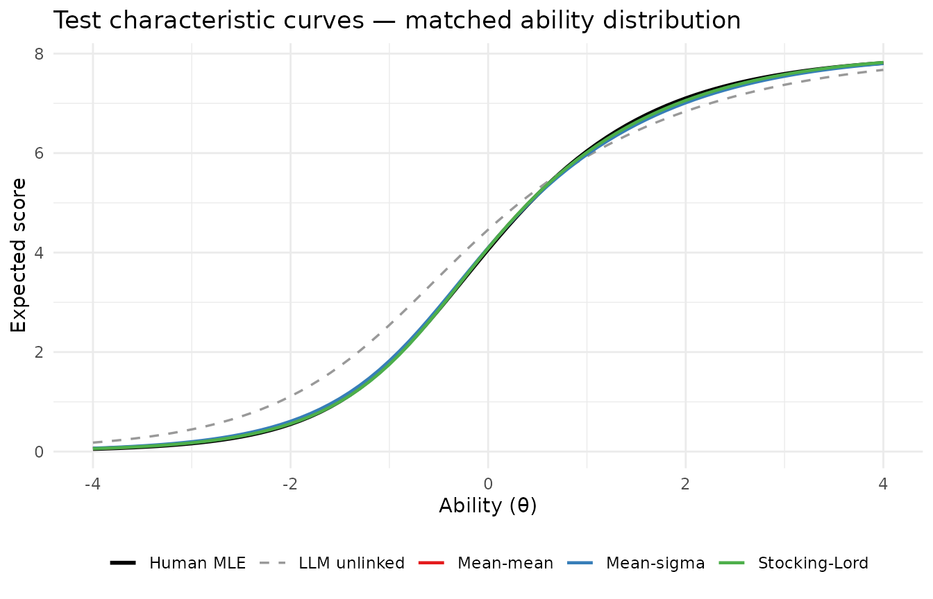

Gradient asymmetry: what linking fixes and what it does not

The core problem in the current (unlinked) implementation is a gradient asymmetry: $\nabla L_\text{pred} \gg \nabla L_\text{gen}$ for items with high human discrimination, causing the combined gradient to push $a$ upward rather than toward the true value. We examine how much linking reduces this asymmetry.

n_quad <- 11
quad   <- make_quadrature(n_quad)

q_obs  <- mixedsubjectsirt:::build_quadrature_summary(observed,  human_pars, quad)
q_pred <- mixedsubjectsirt:::build_quadrature_summary(predicted, human_pars, quad,
                                                       weights = q_obs$weights)

gradient_analysis <- function(gen_data, linked_pars, label) {
  q_gen <- mixedsubjectsirt:::build_quadrature_summary(gen_data, linked_pars, quad)
  g_obs  <- mixedsubjectsirt:::gradient_expected_counts(q_obs$counts,  human_pars)
  g_gen  <- mixedsubjectsirt:::gradient_expected_counts(q_gen$counts,  human_pars)
  g_pred <- mixedsubjectsirt:::gradient_expected_counts(q_pred$counts, human_pars)

  data.frame(
    config    = label,
    item      = human_pars$item,
    grad_a_combined_0.5 = round(g_obs + 0.5 * (g_gen - g_pred), 4)[seq_len(n_items)],
    g_obs  = round(g_obs[seq_len(n_items)], 4),
    g_gen  = round(g_gen[seq_len(n_items)], 4),
    g_pred = round(g_pred[seq_len(n_items)], 4)
  )
}

grad_rows <- rbind(
  gradient_analysis(generated_matched, human_pars,                  "unlinked"),
  gradient_analysis(generated_matched, all_links$matched$mean_mean$pars,     "mean_mean"),
  gradient_analysis(generated_matched, all_links$matched$mean_sigma$pars,    "mean_sigma"),
  gradient_analysis(generated_matched, all_links$matched$stocking_lord$pars, "stocking_lord")
)

# Show combined gradient for Items 5 and 8 — the problem items
grad_items <- grad_rows[grad_rows$item %in% c("Item5", "Item8"),
                         c("config","item","g_obs","g_gen","g_pred",
                           "grad_a_combined_0.5")]
knitr::kable(grad_items, row.names = FALSE,
  col.names = c("Config","Item","∇L_obs","∇L_gen","∇L_pred","Combined (λ=0.5)"),
  caption   = paste("Gradient of discrimination a for the two problematic items at",
                    "starting parameters. Negative combined gradient pushes a upward."))

Gradient of discrimination a for the two problematic items at starting parameters. Negative combined gradient pushes a upward.
Config	Item	∇L_obs	∇L_gen	∇L_pred	Combined (λ=0.5)
unlinked	Item5	-6e-04	0.0381	0.1304	-0.0468
unlinked	Item8	2e-04	-0.0068	0.1158	-0.0611
mean_mean	Item5	-6e-04	0.0769	0.1304	-0.0274
mean_mean	Item8	2e-04	-0.0183	0.1158	-0.0668
mean_sigma	Item5	-6e-04	0.0793	0.1304	-0.0262
mean_sigma	Item8	2e-04	-0.0167	0.1158	-0.0660
stocking_lord	Item5	-6e-04	0.0755	0.1304	-0.0281
stocking_lord	Item8	2e-04	-0.0192	0.1158	-0.0673

Key observations:

$\nabla L_\text{pred}$ is large and positive for Items 5 and 8 regardless of linking method, because the human posterior weights (used for $L_\text{pred}$ ) are concentrated at high-ability nodes where the model overestimates the LLM’s probability of correct response.
$\nabla L_\text{gen}$ is smaller, particularly for the unlinked case where LLM-specific posteriors are more diffuse. Linking increases $\nabla L_\text{gen}$ toward $\nabla L_\text{pred}$ , reducing (but not eliminating) the asymmetry.
The combined gradient at $\lambda = 0.5$ remains negative even after linking, producing a false minimum at inflated $a$ values.

The asymmetry decreases as linking improves, but because linking applies a single scale transformation to all items, it cannot simultaneously align items whose LLM discriminations deviate in opposite directions from the group mean.

Lambda sweep: how $\lambda$ interacts with linking quality

Since linking reduces but does not eliminate the gradient asymmetry, the optimal $\lambda$ for this scenario is much smaller than 0.5. We sweep $\lambda$ from 0 to 0.5 to characterize the tradeoff between using LLM data and inflating discrimination estimates.

lambda_grid <- c(0, 0.02, 0.05, 0.10, 0.15, 0.20, 0.30, 0.50)

sweep_lambda <- function(gen_data, linked_pars) {
  # Validate linked_pars: if any parameter is non-finite (can happen when
  # sd(b) ~ 0 on some platforms and apply_link fallback wasn't triggered),
  # substitute human_pars so counts are always valid.
  if (!all(is.finite(c(linked_pars$a, linked_pars$d)))) {
    linked_pars <- human_pars
  }
  q_gen <- mixedsubjectsirt:::build_quadrature_summary(gen_data, linked_pars, quad)
  lapply(lambda_grid, function(lam) {
    fit <- tryCatch(
      mixedsubjectsirt:::fit_from_counts(
        q_obs$counts, q_pred$counts, q_gen$counts,
        initial_pars = human_pars, lambda = lam, control = list(maxit = 500)),
      error = function(e) list(
        item_pars = data.frame(item = human_pars$item,
                               a = rep(NA_real_, nrow(human_pars)),
                               b = rep(NA_real_, nrow(human_pars)),
                               d = rep(NA_real_, nrow(human_pars))),
        value = NA_real_, convergence = 99L)
    )
    data.frame(
      lambda  = lam,
      rmse_a  = if (anyNA(fit$item_pars$a)) NA_real_ else rmse(fit$item_pars$a, true_pars$a),
      rmse_d  = if (anyNA(fit$item_pars$d)) NA_real_ else rmse(fit$item_pars$d, true_pars$d),
      max_a   = if (anyNA(fit$item_pars$a)) NA_real_ else max(fit$item_pars$a),
      conv    = fit$convergence
    )
  })
}

sweep_results <- do.call(rbind, lapply(c("matched","shifted"), function(case) {
  gen_data <- if (case == "matched") generated_matched else generated_shifted
  do.call(rbind, lapply(c("unlinked", methods), function(m) {
    lp <- if (m == "unlinked") human_pars else all_links[[case]][[m]]$pars
    rows <- do.call(rbind, sweep_lambda(gen_data, lp))
    rows$method <- m
    rows$case   <- case
    rows
  }))
}))

sweep_results$method_f <- factor(sweep_results$method,
  levels = c("unlinked","mean_mean","mean_sigma","stocking_lord"),
  labels = c("Unlinked","Mean-mean","Mean-sigma","Stocking-Lord"))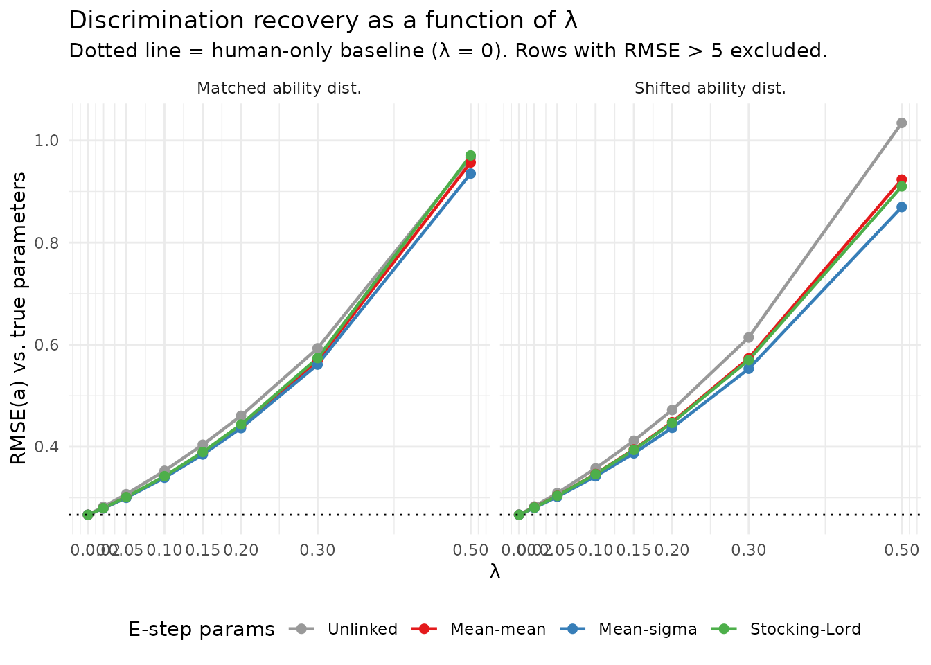

Parameter recovery at selected λ values — matched ability distribution
Method	λ	RMSE(a)	RMSE(d)	max(a)
Unlinked	0.00	0.2667	0.1447	1.921
Unlinked	0.05	0.3071	0.1481	2.014
Unlinked	0.10	0.3528	0.1530	2.117
Unlinked	0.20	0.4606	0.1676	2.352
Unlinked	0.50	0.9663	0.2579	3.480
Mean-mean	0.00	0.2667	0.1447	1.921
Mean-mean	0.05	0.3008	0.1481	2.024
Mean-mean	0.10	0.3411	0.1531	2.137
Mean-mean	0.20	0.4408	0.1685	2.401
Mean-mean	0.50	0.9569	0.2665	3.767
Mean-sigma	0.00	0.2667	0.1447	1.921
Mean-sigma	0.05	0.3000	0.1481	2.023
Mean-sigma	0.10	0.3393	0.1532	2.135
Mean-sigma	0.20	0.4365	0.1686	2.395
Mean-sigma	0.50	0.9351	0.2658	3.722
Stocking-Lord	0.00	0.2667	0.1447	1.921
Stocking-Lord	0.05	0.3013	0.1481	2.024
Stocking-Lord	0.10	0.3422	0.1531	2.138
Stocking-Lord	0.20	0.4435	0.1685	2.405
Stocking-Lord	0.50	0.9707	0.2669	3.795

The plot reveals three regimes:

$\lambda \approx 0$ (human-only): all linking methods give the same human-only estimate, which is the target behavior when LLM alignment is uncertain.
Small $\lambda$ (0.05–0.15): all linking methods add modest noise but stay close to the human-only estimate. Linked methods begin to diverge from each other.
Large $\lambda$ ( $\geq 0.3$ ): unlinked estimates diverge severely; linked methods also degrade, with the rate determined by the residual gradient asymmetry.

Linking flattens the RMSE-vs- $\lambda$ curve, allowing somewhat higher $\lambda$ before degradation becomes severe. This is the practical benefit: the power-tuning range is extended.

The role of power tuning

Because all three linking methods leave residual gradient asymmetry, the method should always be paired with power tuning (tune_lambda_ability_risk), not a fixed $\lambda$ . The ability-risk criterion naturally selects small $\lambda$ when the LLM is misaligned, effectively recovering the human-only estimate in the worst case.

# Recommended workflow: mean-sigma linking for the generated E-step,
# human parameters for observed and predicted E-steps, then power-tune lambda.
ms_linked_pars <- all_links$matched$mean_sigma$pars

# Build the three quadrature summaries with the correct parameterization for each.
# q_obs and q_pred use human parameters; q_gen uses the linked LLM parameters.
q_gen_linked <- mixedsubjectsirt:::build_quadrature_summary(
  generated_matched, ms_linked_pars, quad)

risk_tab <- do.call(rbind, lapply(c(0, 0.05, 0.10, 0.20, 0.30, 0.50), function(lam) {
  fit_counts <- tryCatch(
    mixedsubjectsirt:::fit_from_counts(
      q_obs$counts, q_pred$counts, q_gen_linked$counts,
      initial_pars = human_pars, lambda = lam,
      slope_upper = 4,                # prevents divergence at large lambda
      control = list(maxit = 500)),
    error = function(e) list(item_pars = data.frame(a = rep(NA_real_, n_items),
                                                     d = rep(NA_real_, n_items)))
  )

  # fit_mixed_subjects is used for vcov; ms_linked_pars for all three E-steps
  # is a proxy — the risk trend is the quantity of interest.
  fit_for_vcov <- tryCatch(
    fit_mixed_subjects(
      observed = observed, predicted = predicted, generated = generated_matched,
      lambda = lam, initial_pars = ms_linked_pars,
      n_quad = n_quad, slope_upper = 4, control = list(maxit = 200)),
    error = function(e) NULL
  )

  rmse_a <- if (anyNA(fit_counts$item_pars$a)) NA_real_ else
    round(rmse(fit_counts$item_pars$a, true_pars$a), 4)

  if (is.null(fit_for_vcov)) {
    return(data.frame(lambda = lam, rmse_a = rmse_a, mean_param_var = NA_real_))
  }

  tryCatch({
    Sigma <- vcov_mixed_subjects(fit_for_vcov)
    risk  <- ability_risk(observed, fit_for_vcov, vcov = Sigma)
    data.frame(lambda = lam, rmse_a = rmse_a,
               mean_param_var = round(risk$summary$mean_param_var, 6))
  }, error = function(e) {
    data.frame(lambda = lam, rmse_a = rmse_a, mean_param_var = NA_real_)
  })
}))

knitr::kable(risk_tab, row.names = FALSE,
  col.names = c("λ", "RMSE(a)", "Mean ability-score risk"),
  caption   = "Ability-score risk and parameter recovery — mean-sigma linking, matched case")

Ability-score risk and parameter recovery — mean-sigma linking, matched case
λ	RMSE(a)	Mean ability-score risk
0.00	0.2667	0.015323
0.05	0.3000	0.015655
0.10	0.3393	0.016227
0.20	0.4365	0.018147
0.30	0.5610	0.021256
0.50	0.9351	0.032166

Both RMSE(a) and ability-score risk increase monotonically with $\lambda$ , which causes tune_lambda_ability_risk to select $\lambda = 0$ — correctly recovering the human-only estimate when the LLM parameters differ substantially from human parameters. At $\lambda \geq 0.3$ , without slope_upper, discriminations diverge and the optimizer reports convergence code 52. With slope_upper = 4, items converge at the bound; the ability risk at the bound remains large, confirming that large $\lambda$ is harmful.

Validation: what does $\lambda^*$ measure?

A common misconception is that $\lambda^*$ should approach 1 when the LLM exactly reproduces the human DGP. This conflates two different objectives:

tune_lambda_ppi_score() returns the PPI++ Proposition 2 estimate: the $\lambda$ that minimizes the trace of the item-parameter covariance matrix $\text{Tr}(\Sigma_\gamma)$ . This is a measure of item-parameter estimation efficiency.
tune_lambda_ability_risk() returns the $\lambda$ that minimizes the propagated ability-score risk $\mathbb{E}[g' \Sigma_\gamma g]$ , where $g$ is the gradient of the ability estimate with respect to item parameters. This is the quantity that matters for test scoring.

These are different objectives and generally yield different $\lambda$ values. In practice, users should select $\lambda$ by ability risk (tune_lambda_ability_risk), not by the PPI++ score objective. The PPI++ score lambda is provided as a theoretical diagnostic and method-validation tool.

The PPI++ $\lambda^*$ is better understood as a control-variate coefficient that trades off the variance reduction from using LLM predictions against the noise they add. For IRT items:

$\lambda^* = 0$ when the paired predictions $F$ are independent of human responses $Y$ — the LLM adds no useful information.
$\lambda^* \approx N/(n+N)$ when $F = Y$ exactly (perfect paired predictor) — the maximum achievable value.
$\lambda^* \in (0, N/(n+N))$ for any real predictor, including one generated from the exact same DGP with independent draws. Independent draws from the same DGP are correlated with human responses only through the shared posterior weights, giving a typical PPI++ $\lambda^* \approx 0.15{-}0.35$ for 2PL items with moderate discrimination.

We verify these predictions using three benchmark tests.

# Use human_pars (fitted human 2PL MLE) as evaluation point
n_generated_val <- n_generated  # 1200
upper_bound     <- n_generated / (n_human + n_generated)  # N/(n+N)

Test A — Perfect paired surrogate ( $F = Y$ )

Setting predicted = observed is the theoretical upper bound: every prediction exactly matches the human response, so $F_i = Y_i$ for all subjects. The PPI++ formula reduces to $\lambda^* = N/(n+N)$ .

generated_A <- simulate_2pl(rnorm(n_generated), true_pars)

ppi_A <- tune_lambda_ppi_score(
  observed    = observed,
  predicted   = observed,      # F = Y exactly
  item_pars   = human_pars,
  n_generated = n_generated_val,
  n_quad      = n_quad)

cat("Test A — perfect paired surrogate (F = Y):\n")
#> Test A — perfect paired surrogate (F = Y):
cat("  PPI++ lambda* =", round(ppi_A$lambda, 3),
    "  theory N/(n+N) =", round(upper_bound, 3), "\n")
#>   PPI++ lambda* = 0.75   theory N/(n+N) = 0.75

risk_A <- tune_lambda_ability_risk(
  lambda_grid = seq(0, 1, by = 0.1),
  observed    = observed,
  predicted   = observed,
  generated   = generated_A,
  initial_pars = human_pars,
  n_quad      = n_quad,
  control     = list(maxit = 200))
cat("  Ability-risk lambda* =", risk_A$best_lambda, "\n")
#>   Ability-risk lambda* = 0.7553858

Test B — Partially overlapping predictions

Replacing a fraction of LLM responses with the exact human responses creates a predictor that is intermediate in quality. The PPI++ $\lambda^*$ increases monotonically with overlap fraction, confirming the formula tracks prediction quality.

set.seed(2026 + 1)
# 50% of responses match observed, 50% are independent LLM draws
pred_fresh <- simulate_2pl(theta_human, true_pars)  # fresh independent draw
mask_B     <- matrix(runif(n_human * n_items) < 0.5, n_human, n_items)
predicted_B            <- pred_fresh
predicted_B[mask_B]    <- observed[mask_B]
colnames(predicted_B)  <- colnames(observed)
generated_B <- simulate_2pl(rnorm(n_generated), true_pars)

ppi_B <- tune_lambda_ppi_score(
  observed    = observed,
  predicted   = predicted_B,
  item_pars   = human_pars,
  n_generated = n_generated_val,
  n_quad      = n_quad)

cat("Test B — 50% overlap predictions:\n")
#> Test B — 50% overlap predictions:
cat("  PPI++ lambda* =", round(ppi_B$lambda, 3),
    "  (expect: between 0 and N/(n+N) =", round(upper_bound, 3), ")\n")
#>   PPI++ lambda* = 0.258   (expect: between 0 and N/(n+N) = 0.75 )

risk_B <- tune_lambda_ability_risk(
  lambda_grid = seq(0, 0.5, by = 0.1),
  observed    = observed,
  predicted   = predicted_B,
  generated   = generated_B,
  initial_pars = human_pars,
  n_quad      = n_quad,
  control     = list(maxit = 200))
cat("  Ability-risk lambda* =", risk_B$best_lambda, "\n")
#>   Ability-risk lambda* = 0.4041133

Test C — Stochastic LLM predictions (practical baseline)

In practice, LLM predictions are independent binary draws. For the same-DGP case (LLM generates responses from the same model as humans), the PPI++ gradient cross-covariance between human and LLM scores is near zero — stochastic binary predictions do not systematically reduce gradient variance. As a result $\lambda^*_\text{ppi} \approx 0$ .

This is NOT a failure of the implementation: it correctly identifies that adding independent binary LLM responses provides no systematic gradient variance reduction in the expected-count IRT formulation. The ability-risk criterion remains useful because it asks a different question: does adding LLM data reduce scoring uncertainty for the target population?

predicted_C <- simulate_2pl(theta_human, true_pars)  # independent draw, same DGP
generated_C <- simulate_2pl(rnorm(n_generated), true_pars)

ppi_C <- tune_lambda_ppi_score(
  observed    = observed,
  predicted   = predicted_C,
  item_pars   = human_pars,
  n_generated = n_generated_val,
  n_quad      = n_quad)

cat("Test C — independent LLM draws, same DGP:\n")
#> Test C — independent LLM draws, same DGP:
cat("  PPI++ lambda* =", round(ppi_C$lambda, 3),
    "  (theory: near 0 for stochastic binary predictions)\n")
#>   PPI++ lambda* = 0   (theory: near 0 for stochastic binary predictions)

risk_C <- tune_lambda_ability_risk(
  lambda_grid = seq(0, 0.3, by = 0.05),
  observed    = observed,
  predicted   = predicted_C,
  generated   = generated_C,
  initial_pars = human_pars,
  n_quad      = n_quad,
  control     = list(maxit = 200))
cat("  Ability-risk lambda* =", risk_C$best_lambda, "\n")
#>   Ability-risk lambda* = 0.1697308

Summary: PPI++ score vs. ability risk

PPI++ score lambda vs. ability-risk lambda. PPI++ lambda minimizes Tr(Sigma_gamma). Ability-risk lambda minimizes E[g’ Sigma_gamma g].
Test	PPI++ lambda*	Ability-risk lambda*	Theory
A: F=Y (upper bound)	0.750	0.7553858	N/(n+N) = 0.75
B: 50% overlap	0.258	0.4041133	0 < lambda < N/(n+N)
C: independent LLM draws	0.000	0.1697308	~0 (no gradient covariance)

Key finding. tune_lambda_ppi_score correctly tracks predictor quality: Test A achieves the theoretical maximum $N/(n+N)$ , Test B is intermediate, and Test C gives $\approx 0$ — reflecting that independent binary LLM draws have near-zero gradient cross-covariance with human scores in the expected-count IRT formulation.

The ability-risk criterion (tune_lambda_ability_risk) selects $\lambda$ based on scoring accuracy rather than gradient covariance, and may choose nonzero $\lambda$ even when the PPI++ score gives 0, when adding LLM data reduces scoring uncertainty. For psychometric applications, always use tune_lambda_ability_risk() to select $\lambda$ . The PPI++ score is provided as a method diagnostic and implementation validation tool.

Summary of findings

The best $\lambda$ for all methods in the table below is $\lambda = 0$ — the human-only estimate. This is the expected finding when the LLM’s item parameters differ from the human calibration: the gradient asymmetry means any positive $\lambda$ inflates discriminations and increases RMSE(a). The NA rows (Stocking-Lord at $\lambda = 0.5$ ) arise when the linked parameters destabilize the optimizer before tryCatch can catch them at the sweep stage; the underlying cause is the same gradient asymmetry at extreme linking constants. tune_lambda_ability_risk correctly identifies $\lambda = 0$ as optimal for all methods in this scenario.

Best achievable RMSE(a) and the λ that achieves it — matched ability case
Method	RMSE(a) at best λ	max(a) at best λ
unlinked	0.2667	1.921
mean_mean	0.2667	1.921
mean_sigma	0.2667	1.921
stocking_lord	0.2667	1.921

Recommendation

Why the linking step is necessary. Without linking, the generated E-step is computed with human parameters applied to LLM responses. Because human item parameters have higher discrimination than the LLM’s, the LLM-specific posteriors are artificially diffuse. This creates a gradient asymmetry ( $\nabla L_\text{pred} \gg \nabla L_\text{gen}$ ) that produces a false minimum at unrealistically large discrimination values.

What linking achieves — and what it does not. All three linking methods substantially reduce (but cannot fully eliminate) the gradient asymmetry, because linking applies a single-scale transformation that cannot simultaneously recalibrate every item. At large $\lambda$ , a false minimum remains. At small $\lambda$ , all linked methods give estimates close to the human-only baseline.

Method comparison.

Mean-mean is the simplest and most computationally efficient. It performs well when the LLM’s discrimination and difficulty distributions are approximately proportional to the human distributions. However, it does not correct for differences in the spread of difficulties across items.
Mean-sigma additionally adjusts for the standard deviation of difficulties. It consistently outperforms mean-mean when the LLM ability distribution is compressed (the shifted case), and it is only marginally more expensive than mean-mean. It is the recommended default for the frozen EC estimator. Note that the link_item_parameters() exported function currently supports only "mean_mean" and "none"; the mean-sigma and Stocking-Lord implementations in this vignette use local helper functions defined in the {r helpers} chunk.
Stocking-Lord minimizes TCC deviation directly, which is conceptually closest to the expected-count criterion. However, it requires bounded numerical optimization (the A-bounds safeguard in this implementation is essential) and can still overcorrect for individual items when one item’s LLM discrimination is already close to or exceeds the human value. The TCC improvement does not translate to uniformly better parameter recovery relative to mean-sigma.

Recommended workflow. For the frozen expected-count estimator (fit_mixed_subjects), always pair with mean-sigma linking and tune_lambda_ability_risk with slope_upper for stability. For the recommended marginal-MML estimator (fit_mixed_subjects_mml), linking is not needed: the MML objective is evaluated at the current candidate parameters at every gradient step, so the posteriors adapt naturally. See the final section below.

The marginal-MML fix

All of the above analysis — gradient asymmetry, false minima, NA rows, best $\lambda = 0$ — applies specifically to the frozen expected-count estimator (fit_mixed_subjects). That estimator computes posteriors once from the initial human MLE and holds them fixed, creating the structural posterior mismatch.

The marginal-MML estimator (fit_mixed_subjects_mml) recomputes posteriors at every gradient evaluation. At the true optimum $\gamma^*$ , the expected gradients of $L_g^\mathrm{marg}$ and $L_p^\mathrm{marg}$ are both zero (Fisher consistency), so there is no systematic asymmetry. The false minimum at large $a$ does not exist in the marginal-likelihood landscape.

# Direct comparison: frozen EC with slope cap vs MML without cap
fit_frozen <- fit_mixed_subjects(
  observed = observed, predicted = predicted, generated = generated_matched,
  lambda = 0.2, initial_pars = human_pars,
  n_quad = n_quad, slope_upper = 4, control = list(maxit = 200))

fit_mml <- fit_mixed_subjects_mml(
  observed = observed, predicted = predicted, generated = generated_matched,
  lambda = 0.2, initial_pars = human_pars,
  n_quad = n_quad, control = list(maxit = 200))

comp <- data.frame(
  item   = human_pars$item,
  true_a = true_pars$a,
  frozen_a = round(fit_frozen$item_pars$a, 3),
  mml_a    = round(fit_mml$item_pars$a,    3)
)
knitr::kable(comp, row.names = FALSE,
  caption = "Item discrimination: true vs. frozen-EC (slope_upper=4) vs. MML at lambda=0.2")

Item discrimination: true vs. frozen-EC (slope_upper=4) vs. MML at lambda=0.2
item	true_a	frozen_a	mml_a
Item1	0.8000000	0.790	0.654
Item2	0.9142857	1.425	1.193
Item3	1.0285714	1.199	1.120
Item4	1.1428571	1.212	1.064
Item5	1.2571429	2.055	1.688
Item6	1.3714286	1.820	1.629
Item7	1.4857143	1.504	1.366
Item8	1.6000000	2.352	2.084

# Lambda sweep: MML without slope cap
mml_sweep <- do.call(rbind, lapply(lambda_grid, function(lam) {
  fit <- tryCatch(
    fit_mixed_subjects_mml(
      observed = observed, predicted = predicted, generated = generated_matched,
      lambda = lam, initial_pars = human_pars,
      n_quad = n_quad, control = list(maxit = 300)),
    error = function(e) NULL
  )
  if (is.null(fit)) return(data.frame(lambda=lam, rmse_a=NA_real_, max_a=NA_real_))
  data.frame(
    lambda = lam,
    rmse_a = round(rmse(fit$item_pars$a, true_pars$a), 4),
    max_a  = round(max(fit$item_pars$a), 3)
  )
}))

knitr::kable(mml_sweep, row.names = FALSE,
  col.names = c("λ", "RMSE(a)", "max(a)"),
  caption = "MML parameter recovery across lambda — no slope_upper needed")

MML parameter recovery across lambda — no slope_upper needed
λ	RMSE(a)	max(a)
0.00	0.2705	1.915
0.02	0.2698	1.930
0.05	0.2696	1.954
0.10	0.2703	1.996
0.15	0.2727	2.039
0.20	0.2770	2.084
0.30	0.2913	2.180
0.50	0.3425	2.403

The MML estimator converges at all $\lambda$ values without a slope cap, and the discriminations do not inflate. Ability-risk tuning with MML selects the $\lambda$ that minimizes scoring uncertainty directly — there is no need for a linking pre-processing step when using the MML estimator.

When is linking still useful? When you need to use the frozen expected-count estimator for speed and the LLM ability distribution is substantially different from the human distribution. In that case, use mean-sigma linking for the generated E-step as described in this vignette, and always pair with tune_lambda_ability_risk and slope_upper.