Mixed-Subjects IRT Calibration

This vignette shows the recommended mixed-subjects workflow for a unidimensional 2PL model using the marginal maximum-likelihood (MML) estimator (fit_mixed_subjects_mml). The package expects three item response matrices with no respondent IDs and the same ordering of item columns:

observed: $n$ rows of binary human item responses
predicted: $n$ rows of binary LLM-predicted item responses for the human respondents; rows must be ordered to correspond to respondents in observed
generated: $N$ rows of additional binary LLM-generated item responses (typically $N \gg n$ ), generated from the same model and procedure as predicted

All three matrices must contain binary responses $(Y_{ij} \in \{0,1\})$ . Probability (fractional) predictions are not accepted, as they are not a valid likelihood input for the MML IRT objective and break the correction. If your prediction model outputs probabilities, sample binary responses from them first (e.g. rbinom).

The fitted objective is

$L_o^{\mathrm{marg}}(\gamma) + \lambda\bigl[ L_g^{\mathrm{marg}}(\gamma) - L_p^{\mathrm{marg}}(\gamma)\bigr]$

where $\gamma$ is a vector of item parameters and each $L^\mathrm{marg}$ is the true IRT marginal negative log-likelihood, with posteriors recomputed from the current candidate $\gamma$ at every gradient step. Setting $\lambda = 0$ recovers the human-only MML calibration. See the Choosing Lambda vignette for the specific background on why the MML objective is preferred over expected-count based estimators.

Simulate example data

library(mixedsubjectsirt)
library(ggplot2)

set.seed(242424)

n_human    <- 400
n_generated <- 1200
n_items    <- 8

true_pars <- data.frame(
  item = paste0("Item", seq_len(n_items)),
  a    = seq(0.8, 1.6, length.out = n_items),
  d    = seq(-1.1, 1.1, length.out = n_items)
)
true_pars$b <- -true_pars$d / true_pars$a

theta_human <- rnorm(n_human)
observed    <- simulate_2pl(theta_human, true_pars)

# Strongly informative predictions. On the n labeled subjects, predictions
# match human responses (the F = Y benchmark from the simulation study), and
# N additional unlabeled responses are drawn from the same 2PL. This is
# the "good predictor" regime, where the method should lean on unlabeled data.
# (Further down we show the complementary case of an uninformative predictor,
# where the criterion instead drives lambda to 0.)
predicted <- observed
generated <- simulate_2pl(rnorm(n_generated), true_pars)

Step 1: Fit the human baseline

Baseline models are estimated using mirt.¹

human_start <- fit_2pl(observed, technical = list(NCYCLES = 500))

Step 2: Fit the MML mixed-subjects model

fit_mixed_subjects_mml() uses a MML-based EM procedure for iterative estimation at a given $\lambda$ value. If you have a value of $\lambda$ already (say from a pilot study or previous ability tuning), the model can be estimated directly here.

mixed_mml <- fit_mixed_subjects_mml(
  observed  = observed,
  predicted = predicted,
  generated = generated,
  lambda    = 0.5,
  initial_pars = human_start$pars
)

mixed_mml
#> mixedsubjectsirt 2PL fit
#>   items:      8
#>   lambda:     0.5
#>   loss:       4.91044
#>   convergence: 0 
#>   estimator:  marginal MML PPI++

mixed_mml$item_pars
#>    item         a          d          b
#> 1 Item1 0.7431515 -1.0825772  1.4567382
#> 2 Item2 1.0067308 -0.7278419  0.7229757
#> 3 Item3 0.8547961 -0.4113346  0.4812078
#> 4 Item4 1.0999070 -0.1453192  0.1321195
#> 5 Item5 1.1673630  0.1875514 -0.1606624
#> 6 Item6 1.2566356  0.4923054 -0.3917646
#> 7 Item7 1.5526271  0.8477928 -0.5460376
#> 8 Item8 1.5472343  1.1508445 -0.7438075

Step 3: Select $\lambda$ by ability-score risk

tune_lambda_ability_risk() with fit_fn = fit_mixed_subjects_mml selects the $\lambda$ that minimizes propagated ability-score risk $\mathbb{E}\big[g'\Sigma_\gamma g\big]$ (where $\Sigma_\gamma$ is the Louis-corrected marginal sandwich covariance).² By default this is done by direct 1-D optimization over [0, 1]. The final fit from this optimal $\lambda$ is also returned as the best_fit object within the output list, so the user is not required to call fit_mixed_subjects_mml again.

ability_tuned <- tune_lambda_ability_risk(
  observed     = observed,
  predicted    = predicted,
  generated    = generated,
  target_resp  = observed,
  initial_pars = human_start$pars,
  fit_fn       = fit_mixed_subjects_mml,
  control      = list(maxit = 200)
)

ability_tuned$best_lambda
#> [1] 0.7924548

Because the predictor is highly informative, the approach selects a $\lambda$ near the theoretical maximum $N/(n+N) = 1200/1600 = 0.75$ . As such, the method leans heavily on the unlabeled response data. (The returned summary records each $\lambda$ the optimizer evaluated, with selection_risk = Inf for any that failed to converge, so selection is protected against numerical failures. When the predictor is uninformative the same criterion drives $\lambda$ to 0 instead; see below.)

Step 3b (recommended workflow): cross-fit $\lambda$ tuning

tune_lambda_ability_risk() above estimated an appropriate $\lambda$ and fits the final model on the same data used for this estimation. Previous analysis of prediction-powered inference in finite samples shows that estimating $\lambda$ on the data you also estimate model parameters with is optimistic. Item parameters estimated this are biased in finite samples and may undercover true parameter values.³

tune_lambda_ability_risk_crossfit() removes this bias by tuning $\lambda$ on held-out data: each fold’s $\lambda$ is chosen using only out of fold item responses, and the final fit combines them. Passing fit_fn = fit_mixed_subjects_mml for the per-fold tuning and final_fit_fn = fit_mixed_subjects_mml for the final fit produces a single scalar- $\lambda$ mixed subjects calibration fit (the fold-specific $\lambda$ ’s are averaged, weighted by fold size).

cf_tuned <- tune_lambda_ability_risk_crossfit(
  observed     = observed,
  predicted    = predicted,
  generated    = generated,
  initial_pars = human_start$pars,
  fit_fn       = fit_mixed_subjects_mml,
  final_fit_fn = fit_mixed_subjects_mml,
  n_splits     = 2,          # the standard PPI sample split (also the default)
  control      = list(maxit = 200)
)

cf_tuned$lambda_by_split   # one tuned lambda per held-out fold
#> [1] 0.8758023 0.8896977
cf_tuned$lambda_final      # fold-size-weighted scalar used for the final fit
#> [1] 0.88275

The object cf_tuned$final_fit provides the final model fit from calibration, and vcov(cf_tuned$final_fit) gives its Louis-corrected covariance. We suggest use of the default n_splits = 2, the standard PPI sample split (one half tunes, the other estimates, then swap). You may notice the cross-fit $\lambda$ (here $\approx 0.85$ ) sits above the same-data value ( $\approx 0.7$ ) and above the perfect-predictor ceiling $N/(n+N) = 0.75$ . That is expected and is not evidence of a better $\lambda$ : with two folds each $\lambda$ is tuned on only half the labeled subjects ( $n_\text{train} = n/2 = 200$ ), and the PPI-optimal $\lambda$ grows as labeled data shrinks (it tracks $N/(N + n_\text{train})$ , here $1200/1400 \approx 0.86$ ). The fold $\lambda$ ’s are tuned for $n_\text{train}$ but the final fit applies their average to the full sample, so they run a little higher than $\lambda$ estimated in the same sample; in operational settings where $N \gg n$ , this difference shrinks to zero. Importantly, the reason to cross-fit is not the $\lambda$ value, but to remove finite-sample item parameter bias. The cheaper same-data tuner in Step 3 is fine for exploration; prefer the cross-fit estimate for operational calibrations or further research.

Step 4: Inspect the covariance

vcov() on a scalar-lambda MML fit automatically uses vcov_mixed_subjects_mml(), which applies Louis’ observed-information correction.⁴ Here, the bread is $H_\mathrm{comp} - I_\mathrm{miss}$ rather than the EM complete-data Hessian alone.

Sigma <- vcov(cf_tuned$final_fit)
dim(Sigma)  # 2J × 2J
#> [1] 16 16

Compare calibrations

human_only <- fit_mixed_subjects_mml(
  observed  = observed,
  predicted = predicted,
  generated = generated,
  lambda    = 0,
  initial_pars = human_start$pars
)

estimates <- rbind(
  data.frame(estimator = "human only",  human_only$item_pars),
  data.frame(estimator = "MML lambda = 0.5", mixed_mml$item_pars),
  data.frame(estimator = "MML ability-risk",
             ability_tuned$best_fit$item_pars)
)
estimates$true_b <- true_pars$b[match(estimates$item, true_pars$item)]
estimates$true_a <- true_pars$a[match(estimates$item, true_pars$item)]

ggplot(estimates, aes(true_b, b, colour = estimator)) +
  geom_abline(slope = 1, intercept = 0, linewidth = 0.4) +
  geom_point(size = 2) +
  labs(x = "True difficulty", y = "Estimated difficulty", colour = NULL) +
  theme_minimal()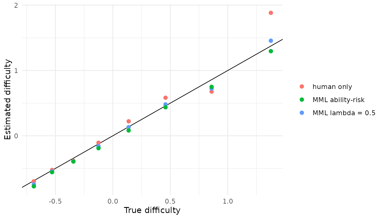

When the LLM is uninformative

While the method is able to efficiently exploit information derived from a good predictor, it is also capable of rejecting useless information derived from a bad one. Here we simulate responses that are essentially unrelated to ability (drawn from scrambled item parameters), so the paired correction between observed and predicted carries no usable signal:

set.seed(242424)
bad_pars    <- true_pars
bad_pars$a  <- pmax(0.05, abs(rnorm(n_items, 0, 0.1)))   # near-zero slopes
bad_pars$d  <- rnorm(n_items, 0, 2)                       # difficulties unrelated to truth

predicted_bad <- simulate_2pl(theta_human, bad_pars)
generated_bad <- simulate_2pl(rnorm(n_generated), bad_pars)

tuned_bad <- tune_lambda_ability_risk(
  observed     = observed,
  predicted    = predicted_bad,
  generated    = generated_bad,
  target_resp  = observed,
  initial_pars = human_start$pars,
  fit_fn       = fit_mixed_subjects_mml,
  control      = list(maxit = 200)
)

tuned_bad$best_lambda   # expect ~0: the useless LLM is correctly ignored
#> [1] 0.03332212

The criterion drives $\lambda \to 0$ , recovering the human-only item parameters. As such, the same $\lambda$ tuning procedure both embraces informative predictions (as in the main example, $\lambda \to N/(n+N)$ ) and rejects an uninformative predictions ( $\lambda \approx 0$ ).

Validation

A full simulation study confirms the recommended workflow behaves as intended:

$\mathbf{\lambda}$ -selection tracks predictor quality. A perfect paired predictor $(F = Y)$ selects $\lambda \approx N/(n+N)$ ; a useless predictor is down-weighted to $\lambda \approx 0$ .
The Louis-corrected standard errors provide correct coverage. Across all simulation conditions, including a useless or biased predictor, vcov() on a scalar MML fit attains nominal Wald-interval coverage (~0.91/0.96) for both discriminations and intercepts, whereas the uncorrected EM-Hessian covariance under-covers (~0.71/0.79).
No average harm done to ability scoring. The tuned ability-score RMSE is no worse than the human-only calibration on average (every regime’s mean $\Delta \text{RMSE} \leq 0$ ) when the predictor is uninformative.

See the Simulation Validation vignette for the full results, and simulations/ in the source tree for the reproduction code.