Calibrating with a Weakly-Informative, Biased LLM

This vignette treats the regime prediction-powered inference is built for: a smaller human sample (here n = 500) alongside a much larger synthetic / LLM sample (N = 100000). The LLM here is biased, in that its item parameters are systematically off, making them only weakly informative about the human responses.

Importantly, the mixed-subjects (PPI) estimator is asymptotically unbiased for the true human parameters at every $\lambda$. Tuning $\lambda$ is an efficiency knob, not a bias knob. A naive fit that pools the human and LLM responses has no such protection: the n = 500 humans are outvoted by the N = 100000 rows of LLM-generated responses, and the estimate inherits the LLM’s biased data generating process.

All numbers are precomputed (data-raw/precompute_largeN.R): n = 500, N = 100000, 16 Monte Carlo replications.

The setup

Human responses come from a true 8-item 2PL model (a ∈ [0.8, 1.6], d ∈ [-1.1, 1.1]). The LLM is a shifted version with discriminations attenuated by 10% and intercepts shifted up by 0.25. This makes the response structure plausible but biased:

true_pars <- data.frame(item = paste0("Item", 1:8),
                        a = seq(0.8, 1.6, length.out = 8),
                        d = seq(-1.1, 1.1, length.out = 8))
llm   <- true_pars
llm$a <- 0.9 * true_pars$a       # ~10% attenuated discriminations
llm$d <- true_pars$d + 0.25      # +0.25 intercept shift

theta     <- rnorm(500)
observed  <- simulate_2pl(theta, true_pars)             # n = 500 human
predicted <- simulate_2pl(theta, llm)                   # paired LLM (same people)
generated <- simulate_2pl(rnorm(100000), llm)           # N = 100000 unlabeled LLM

Naive pooling inherits the bias

The obvious move is to pool everything and fit one model:

naive <- fit_2pl(rbind(observed, generated))   # 500 human + 100000 LLM rows

The 500 humans are in the fit, but against 100,000 LLM rows their information is washed out, and the estimate is dragged onto the LLM’s shifted parameters:

Averaged over the replications, the naive estimator’s item-parameter bias is -0.119 in the slopes and +0.248 in the intercepts — essentially the LLM’s shift (−0.1·a, +0.25). Because N = 100000, that wrong answer is estimated very precisely (a tiny standard error); more LLM data only sharpens the bias.

$\lambda$ moves efficiency, not bias

The mixed-subjects estimator minimizes the loss

$$L_o^{\mathrm{marg}}(\gamma) \;+\; \lambda\bigl[L_g^{\mathrm{marg}}(\gamma) - L_p^{\mathrm{marg}}(\gamma)\bigr].$$

At the true parameters the human loss is mean-zero and the paired correction L_g − L_p is also mean-zero, so the estimating equation is mean-zero for every $\lambda$. Unbiasedness comes from this structure, not from a specific value of $\lambda$. To see it directly, we fit the estimator across a grid of $\lambda$ values and track two things: the item-parameter bias (Monte Carlo mean of estimate − truth) and the model-based ability-score risk $\mathbb{E}\big[g'\Sigma_\gamma(\lambda) g\big]$ (the quantity the tuner actually minimizes).

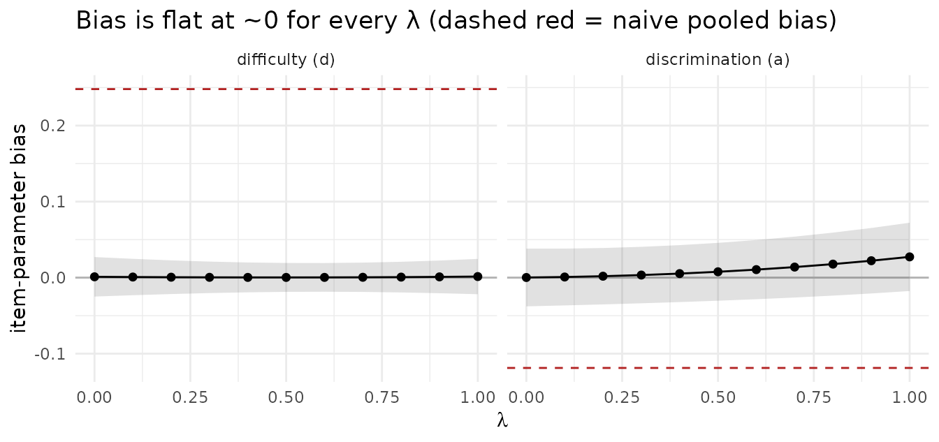
The mixed-subjects bias sits on zero across the entire range of $\lambda$ (the shaded band is $\pm 2$ Monte Carlo SE); the dashed red lines mark the naive pooled bias. Tuning $\lambda$ changes efficiency:

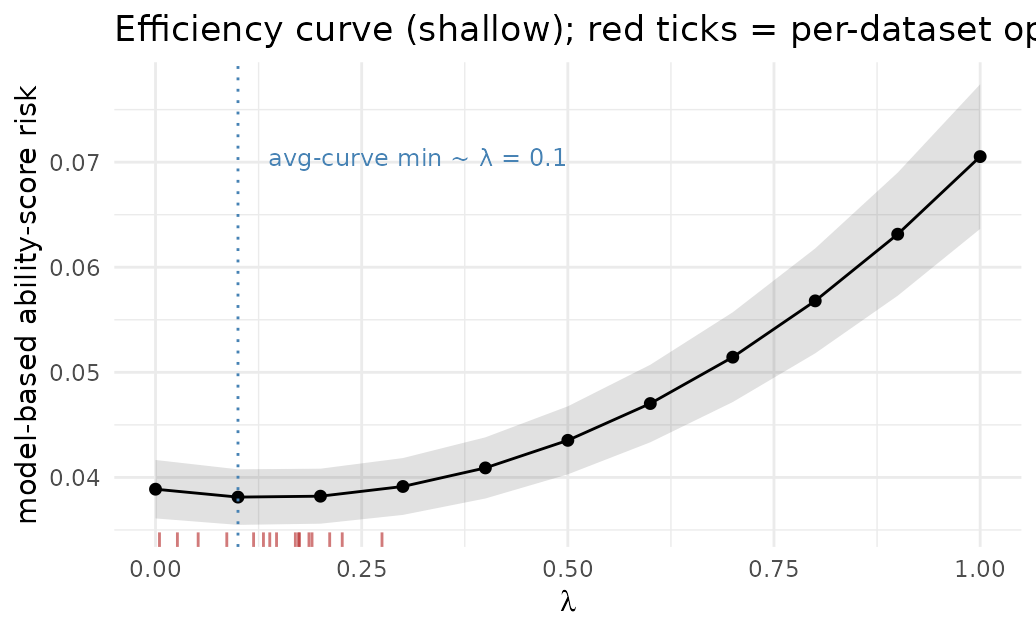
For this weakly-informative LLM the averaged risk curve is shallow and rises for larger λ: leaning on a poorly-correlated predictor adds measurement error to latent ability. Its minimum sits near λ ≈ 0.1, onlyabout 2% below the λ = 0 (human-only) risk — almost no efficiency to begained. Because the curve is so flat, each individual dataset’s optimum scatters around this value (the red ticks); see the next section. Every pointon the curve is unbiased.

Choosing $\lambda$

The curve above was sampled on a grid only to draw the surface using tune_lambda_ability_risk(..., method = "grid"). To choose an operating $\lambda$ you do not need a grid at all. By default, tune_lambda_ability_risk() selects $\lambda$ by direct optimization of the risk over [0, 1] (stats::optimize()):

# Direct optimization is the default (method = "optimize").
tuned <- tune_lambda_ability_risk(
  observed = observed, predicted = predicted, generated = generated,
  target_resp = observed, initial_pars = human_start$pars,
  fit_fn = fit_mixed_subjects_mml, n_quad = 11
)
tuned$best_lambda            # continuous lambda

# Pass method = "grid" (and a lambda_grid) to scan instead -- how the curve
# above was drawn. lambda_grid otherwise just bounds the optimizer's search.

The optimizer returns the minimizer of this dataset’s risk surface. Here, λ = 0.27. Every dataset has its own (noisy) risk surface, so its optimal λ varies. Across the 16 replications the per-dataset optimum averaged 0.14 and ranged [0.0, 0.3], scattering around the minimum of the averaged curve (≈ 0.1). (These are not the same point — the minimum of the average risk is not the average of the per-dataset minima.) The scatter is wide here because the surface is shallow; informative predictions sharpens it.

(The 2-fold cross-fitted tuner, tune_lambda_ability_risk_crossfit(), lands at the same place: at $N \gg n$ the cross-fit $\lambda$-inflation $N/(N + n/2)$ vs $N/(N + n)$ is negligible, so cross-fitting does not change the selected $\lambda$.)

Takeaways

1. The mixed-subjects estimator is unbiased for the true human parameters at every $\lambda$; pooling lets a large biased LLM sample outvote the human anchor and inherits its bias.
2. $\lambda$ tuning is performed directly and efficiently. tune_lambda_ability_risk() selects $\lambda$ by direct 1-D optimization by default; a grid (method = "grid") is just a convenient way to visualize the whole risk surface.

Reproducing

data-raw/precompute_largeN.R runs the Monte Carlo over the λ grid and the direct optimization, and writes the cached results (Rscript data-raw/precompute_largeN.R [n_reps] [cores] [N]). At N = 100000 each fit takes several seconds, so it is run once offline rather than during vignette knitting; pass a larger N to confirm the picture is unchanged.